
Backtesting liquidity algorithms is how decentralized finance (DeFi) protocols test strategies using past blockchain data. It helps liquidity providers (LPs) evaluate risks, like impermanent loss, and potential returns from trading fees. Unlike traditional finance, DeFi backtesting focuses on modeling token reserves and fee dynamics in liquidity pools, especially for advanced setups like Uniswap V3‘s concentrated liquidity.
Key insights:
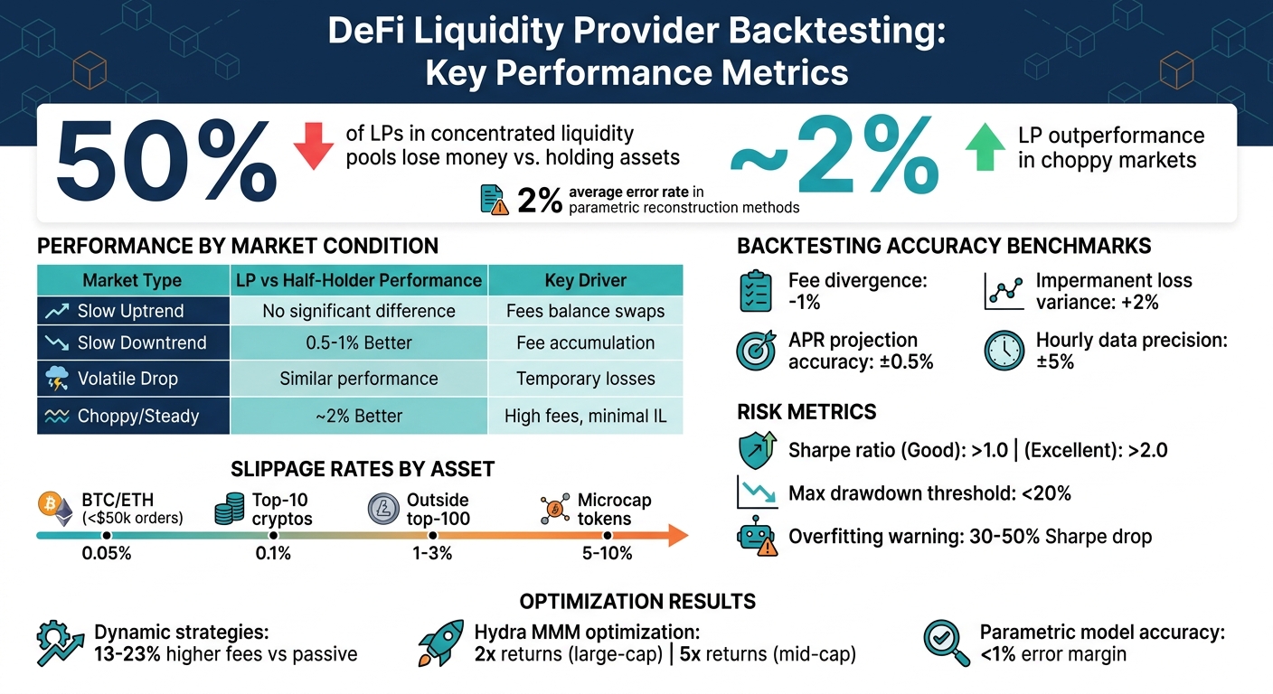
- Concentrated Liquidity Risks: Nearly 50% of LPs in these pools lose money compared to just holding assets.
- Essential Tools: Building a backtesting framework requires granular swap data, liquidity pool models, and simulations that factor in gas fees, slippage, and network conditions.
- Performance Metrics: LP strategies often outperform simple holding in choppy markets by ~2%, but results heavily depend on market conditions and strategy precision.
- Practical Challenges: Gas costs, slippage, and incomplete historical data can impact accuracy. Advanced methods, like parametric reconstruction, help rebuild liquidity states with ~2% error.
DeFi Liquidity Provider Performance: Key Backtesting Metrics and Market Outcomes
Core Elements of a Backtesting Framework
This framework is built on three main components: accurate pool models, detailed historical data, and realistic market simulations. Each piece addresses distinct challenges in decentralized protocol environments.
Modeling Liquidity Pools
To start, you need a precise understanding of how liquidity pools function. For Uniswap V2, this means implementing the constant product formula ($x \cdot y = k$), where the product of token reserves remains constant during swaps. However, Uniswap V3 and other concentrated liquidity protocols demand a more advanced approach. These protocols use a liquidity-state function $\mathcal{V}(L, p, B)$ to map liquidity ($L$) and price ($p$) within a specific range ($B$) to token reserves.
Concentrated liquidity adds complexity by dividing the price axis into equal-width buckets, tracking how liquidity moves between active and inactive states as prices change. Incomplete historical snapshots make this even trickier. For example, in October 2024, researchers Andrey Urusov, Rostislav Berezovskiy, and Yury Yanovich developed a framework for Uniswap V3 that used multi-dimensional NumPy arrays with GPU acceleration. Later, in March 2026, the Vega Institute Foundation introduced a "parametric reconstruction" method to rebuild historical liquidity states from swap data, achieving an average error rate of around 2%.
To maintain accuracy, each swap, mint, and burn event must be tracked to update liquidity provider (LP) token ratios and fees, such as Uniswap V2’s 0.3% fee structure.
Once the pool model is set, the next step is gathering granular historical data to fuel simulations.
Gathering Historical Price and Volume Data
For concentrated liquidity protocols, aggregated data (like minute or hourly-level updates) isn’t detailed enough. Instead, you’ll need swap-level data that includes price updates and trade volumes, capturing bidirectional flows often missed in aggregated datasets.
| Data Type | Source Examples | Purpose in Backtesting |
|---|---|---|
| Swap Transactions | The Graph, Archive Nodes | Reconstructing price paths and trade volumes |
| Liquidity Snapshots | Amberdata API, Revert.finance | Tracking pool depth and LP token ratios |
| On-Chain Metrics | Glassnode, Dune Analytics | Monitoring TVL flows and wallet activity |
| Gas Fee History | Etherscan | Factoring in network costs for profit modeling |
The Graph allows you to download swap and hourly liquidity data for specific pools. For the highest precision, Web3 archive nodes can query historical liquidity states at the block level. Providers like Amberdata simplify tracking by offering snapshots for every swap, mint, and burn event.
Combining swap data with liquidity snapshots lets you pinpoint active liquidity at the exact moment of each transaction. Using The Graph’s hourly data for simpler positions achieves a precision of approximately +/-5%, verified by tools like Revert Finance.
Recreating Market Conditions
With accurate pool models and granular data in place, the final step is simulating real-world market conditions to account for execution challenges.
Factors like gas fees and slippage can significantly impact returns. Gas costs vary with network congestion, while slippage occurs when trades shift prices in less liquid pools. To address this, set maximum slippage tolerances and integrate real-time gas costs into your backtesting setup.
Another key factor is impermanent loss, which measures the difference between holding assets in a pool versus holding them outside of it. For example, in May 2021, a real-world Uniswap V3 position managed by ameen.eth in the ETH/USDC 0.3% fee pool demonstrated the effectiveness of a backtesting framework. Starting with approximately $481,000 (251,271 USDC and 229,696 ETH) at a price range of $1,844.61 to $2,858.36, the backtest showed only -1% divergence in accrued fees and +2% for impermanent loss compared to actual results. This confirmed that even hourly data could project APR within 0.5% of real outcomes.
As Andrey Urusov of the Vega Institute Foundation put it:
"The core innovation lies in reconstructing historical liquidity states from readily available swap data, enabling rigorous strategy development without dependency on historical liquidity snapshots."
Before deploying actual funds, it’s wise to conduct "paper trading." This step tests strategy execution in a live environment without financial risk, revealing potential gaps in your backtesting model.
sbb-itb-7e716c2
Building Your Backtesting Environment
Once you’ve laid the groundwork, the next step is to bring your theoretical models to life by creating a functional simulation environment. This involves integrating the right tools and configurations to transform abstract concepts into actionable setups.
Selecting Tools and Infrastructure
Python is the backbone of most backtesting frameworks, and for good reason. Its libraries, like Pandas for time-series data and NumPy for mathematical operations, are perfect for handling the complex data requirements of liquidity modeling.
A solid data infrastructure is non-negotiable. For historical swap and liquidity data, The Graph provides decentralized subgraphs that allow you to retrieve specific pool data. If you need block-level precision, a Web3 archive node is indispensable – it lets you query historical liquidity states at every block, which is especially critical for protocols like Uniswap V3 that use concentrated liquidity.
For additional data needs, APIs from providers like Amberdata, Glassnode, and Dune Analytics offer access to historical price, volume, and on-chain metrics. Want to factor in gas fees? Etherscan is a great resource for historical gas data, which can help you gauge how network costs might impact profitability.
When dealing with millions of data points, CPU performance may not cut it. That’s where GPU-accelerated libraries like CuPy come in, providing the speed needed for large-scale simulations.
| Tool/Infrastructure | Purpose | Example Providers |
|---|---|---|
| Data Querying | Fetching on-chain swap/liquidity events | The Graph, Dune Analytics |
| Historical Metrics | Price, OHLCV, and TVL flows | Glassnode, CryptoCompare, Amberdata |
| Execution Modeling | Calculating net profit after network costs | Etherscan (gas history), DexGuru |
| Computational Libs | Numerical analysis and GPU acceleration | NumPy, CuPy, Pandas |
Setting Up Liquidity Algorithm Parameters
With the tools ready, the next step is configuring your algorithm to align with your market strategy. Begin by defining price ranges – the upper and lower bounds (ticks) for concentrated liquidity positions. These ranges determine where your capital is deployed and directly affect its efficiency.
Then, choose a fee tier for the pool you’re testing. Uniswap V3, for example, offers multiple fee tiers such as 0.05%, 0.3%, and 1%. Stablecoin pools generally use lower fees, while volatile pairs benefit from higher tiers to compensate for the added impermanent loss risk. For dynamic strategies, establish rebalancing rules that dictate when and how to adjust positions based on price changes.
Other critical parameters include initial capital, token ratios, and slippage tolerance. To model execution costs, integrate gas price data to account for transaction overhead. As Andrey Urusov from the Vega Institute Foundation explains:
"Precise modeling requires the full sequence of in-pool price updates generated by every swap during the modeling period, together with the corresponding trade volumes."
Lastly, determine the protocol environment for your simulation – whether it’s Ethereum mainnet, Optimism, Arbitrum, or Polygon. Each chain has unique gas costs and block times, which can influence your results. To avoid overfitting your strategy, test it across various market conditions (uptrend, downtrend, and sideways trends) to ensure it performs consistently.
Interpreting Backtesting Results
Building on the simulated market conditions discussed earlier, it’s time to turn those results into actionable insights. The key is to assess whether your liquidity algorithm can handle real market scenarios effectively.
Measuring Performance
Here’s a summary of how liquidity provider (LP) performance varies across different market conditions:
| Market Condition | LP Performance vs. Half-Holder | Key Driver |
|---|---|---|
| Slow Uptrend | No significant difference | Fees balance out ETH being swapped for USDC |
| Slow Downtrend | 0.5% – 1% Better | Fee accumulation offsets the price drop |
| Volatile Drop | Similar to Half-Holder | Losses could be temporary if the price rebounds |
| Choppy/Steady | ~2% Better | High fee collection with minimal impermanent loss (IL) |
Performance is best measured by Net Profit and Loss (PnL) – the total of fees earned minus impermanent loss and costs like gas fees. This metric gives you the net outcome of your strategy. Compare your LP performance against a half-holder strategy (50/50 split between assets) rather than a full-holder, as LP strategies inherently require splitting capital.
For instance, Amberdata’s backtesting of an LP strategy in the Uniswap V2 ETH/USDC pool during a slow downtrend (March–June 2022) revealed that the LP approach outperformed a half-ETH/half-USDC holder by 0.5% to 1% in 95% of cases. This was mainly due to fee accumulation offsetting ETH’s 33% price decline.
Another critical measure is capital efficiency, calculated as trading volume divided by Total Value Locked (TVL). For example, Uniswap V2’s DAI/USDT pool showed 400% higher capital efficiency compared to the DAI/USDC pool, as fewer providers competed for fees in the DAI/USDT pool.
For strategies involving concentrated liquidity, such as Uniswap V3, monitor the active liquidity percentage – the proportion of time the market price stayed within your set range. If this percentage is low, your capital isn’t generating returns.
Don’t overlook risk-adjusted returns. The Sharpe ratio is a helpful indicator, with values above 1.0 considered decent for crypto and above 2.0 being excellent. Also, track maximum drawdown, which measures your largest loss from peak to trough; effective strategies generally keep this below 20%.
Comparing and Refining Strategies
To fine-tune your approach, test multiple strategies to balance fee earnings against impermanent loss. Compare passive wide-range strategies with dynamic narrow-range ones, experiment with different fee tiers, and test varying rebalancing frequencies. Backtests of Uniswap V3 strategies revealed that narrow, dynamic ranges using Bollinger Bands often underperformed wider, passive ranges, as higher fees couldn’t offset greater impermanent loss and gas costs from frequent rebalancing.
As JNP from Coinmonks aptly put it:
"The main enemy of an active liquidity provider is the accumulation of impermanent loss and not the accumulation of gas costs"
Use walk-forward analysis with rolling windows (e.g., 6 months for training, 1 month for testing) to identify overfitting. A Sharpe ratio drop of 30-50% between in-sample and out-of-sample data is a clear warning sign.
Test strategies across various market conditions – uptrend, downtrend, volatile, and choppy markets. Liquidity provision tends to excel in choppy markets, where prices oscillate without a clear trend, often outperforming a half-holder strategy by around 2%. Amberdata’s research supports this:
"In every scenario but extremely downward trending markets, our liquidity provider strategy performed better than a holder of half ETH and half USDC"
For protocols like Hydra Market Making, which use oracle-informed pricing, iterative testing can optimize parameters. Backtests showed that adjusting the ‘c’ parameter (balancing LP compensation and arbitrage incentives) significantly boosted returns – over 2x for large-cap tokens like BTC and ETH, and up to 5x for mid-cap tokens compared to standard AMMs. Typically, a ‘c’ value of 1.25 works well for large-cap tokens, while mid-caps benefit from a more cautious 1.5.
Finally, always prepare for the worst. Simulate pessimistic scenarios by doubling historical spread penalties, adding 100-200ms execution delays, and modeling realistic slippage – 0.05% for top-tier coins and up to 10% for microcaps. The goal isn’t just finding a profitable backtest but ensuring your strategy can withstand real-world challenges.
Best Practices for Real-World Application
Before deploying your algorithm in live trading, it’s essential to test it against the toughest market scenarios. Many strategies falter in the leap from simulation to live trading, so ongoing adjustments are key to staying effective.
Testing Under Extreme Conditions
Run your strategy against historical market crashes, such as March 2020, May 2021, and the FTX collapse. These stress tests help reveal whether your algorithm can withstand extreme volatility and liquidity shortages while protecting capital.
When testing under high-stress conditions, factor in significant slippage rates. For instance:
- Apply 0.05% slippage for BTC and ETH on orders below $50,000.
- Use 0.1% slippage for top-10 cryptocurrencies.
- Increase to 1–3% slippage for tokens outside the top 100.
- For microcap tokens, prepare for 5–10% slippage.
A stark example occurred in January 2024, when a $9 million market order for the dogwifhat (WIF) token resulted in a $5.7 million loss (a 63% drop) due to a thin order book.
To further stress test your model, introduce execution delays and spread penalties. Add 100–200 milliseconds of latency to simulate real-world conditions and double historical spread averages, including full taker fees. As tech journalist Olha Svyripa points out:
"The goal isn’t finding a profitable backtest, it’s finding one that survives pessimistic assumptions".
If your Sharpe ratio drops by more than 30–50% when moving from training to test datasets, it’s a clear sign of overfitting. Once your strategy proves durable under these conditions, focus on refining it to adapt to evolving markets.
Continuous Improvement Process
Markets change rapidly, and your algorithm must keep up. After passing stress tests, implement a continuous improvement cycle. Use walk-forward analysis with rolling windows – optimize on six months of data, then test on the following month – to prevent your algorithm from simply memorizing historical patterns.
Before going live, validate your algorithm in a sandbox or testnet environment for at least 30 days. This ensures proper API connectivity, fee calculations, and execution logic without risking real funds. When transitioning to live trading, start small – allocate just 5–10% of your intended capital for the first 30 days. Only scale to full capital after 60 days of live performance that aligns within 20% of your backtest projections.
Lastly, monitor performance regularly and re-run backtests every quarter using fresh data. This helps you detect shifts in market conditions and adjust parameters as needed to maintain effectiveness.
How BeyondOTC Supports Backtesting and Liquidity Optimization

Building a strong backtesting framework takes more than just algorithms – it demands reliable technical infrastructure, precise market data, and deep liquidity insights. BeyondOTC’s TVL funding advisory equips DeFi projects with the tools to reconstruct historical liquidity states and validate how their algorithms perform under different conditions.
Total Value Locked (TVL) acts as a crucial benchmark for recreating historical pool depths. Through its network, BeyondOTC provides access to accurate TVL data across active price ranges, enabling algorithms to estimate liquidity levels dynamically within operational ranges. This precise TVL data becomes the backbone of collaborations that refine backtesting approaches.
BeyondOTC also connects DeFi protocols with liquidity providers and institutional investors, offering quantitative assessments of returns and risks. This allows teams to simulate τ‐strategies and concentrated liquidity positions, striking a balance between capital efficiency and minimizing impermanent loss. In fact, crypto strategies backed by structured backtesting frameworks have shown annualized excess returns of up to 8.76%.
Moreover, BeyondOTC supplies historical swap data and detailed liquidity snapshots that capture every mint, swap, and burn event within liquidity pools. This granular data is key for reconstructing historical liquidity states, enabling projects to calculate fees and impermanent loss without needing to track individual LP tokens. By using parametric reconstruction methods, teams can rebuild historical liquidity profiles solely from swap sequences.
When it’s time to move from testing to deployment, BeyondOTC’s network offers capital deployment channels through OTC desks, market makers, and institutional investors. Covering centralized exchanges, decentralized exchanges, and specialized liquidity providers, this network ensures projects have multiple options to optimize liquidity management based on their backtested results. With access to such detailed data and robust capital channels, BeyondOTC helps projects transition smoothly from backtesting to live liquidity strategies that are both effective and resilient.
Conclusion
Backtesting liquidity algorithms shifts capital deployment from guesswork to a data-driven approach. By turning liquidity provision into a more active process, backtesting allows you to evaluate potential returns, assess impermanent loss, and identify the strategies that thrive in actual market conditions.
For instance, dynamic strategies, when fine-tuned, can yield 13–23% higher fees than passive benchmarks, while parametric models predict rewards with an error margin of less than 1%. However, research highlights a stark reality: nearly 50% of liquidity providers end up losing money compared to simply holding their assets. On the flip side, in volatile markets, liquidity providers can outperform asset holders by roughly 2%.
To start, reconstruct historical liquidity states using detailed swap transaction data while accounting for factors like gas fees and slippage. Avoid relying on aggregated snapshots; instead, use high-granularity data for precision. Test your strategies across different market scenarios – whether oscillating, trending, or volatile – to pinpoint where they shine and where they might stumble. Once you’ve refined your approach, validate it through forward testing with smaller investments before scaling up.
The most successful protocols view backtesting as an ongoing process, not a one-time task. By consistently applying and refining these methods, you can develop liquidity strategies that are efficient with capital and resilient under varying market conditions. Use these practices to strengthen your DeFi protocol and build strategies that stand the test of time.
FAQs
How do I backtest Uniswap V3 liquidity without historical snapshots?
To backtest Uniswap V3 liquidity, you can reconstruct liquidity states using swap transaction data. This approach eliminates the need for historical snapshots by relying on parametric models or tools to estimate liquidity ranges and pool conditions. By analyzing transaction data, you can simulate pool states effectively, allowing for precise backtesting of liquidity strategies while keeping errors to a minimum.
What data granularity is needed for accurate LP backtesting?
When it comes to backtesting liquidity provider (LP) strategies in DeFi protocols, data granularity plays a huge role in accuracy. While many rely on daily data, using more detailed data – like hourly or even minute-level information – can drastically refine precision.
Granular data provides insights into transaction-level activity, such as swap events and changes in liquidity. This level of detail allows for a more accurate reconstruction of historical liquidity states. By capturing dynamic market behaviors, it ensures that LP strategy modeling reflects the real-world activity over time, leading to better-informed decisions.
How should I model gas fees and slippage in my simulations?
To accurately model gas fees and slippage, it’s important to base your assumptions on real-world market conditions. This means factoring in transaction fees (like taker fees) and accounting for dynamic slippage, which depends on liquidity and the size of the order.
You can simulate costs by incorporating either a percentage-based fee or a fixed fee per trade. For slippage, use historical data or market impact models to reflect how trades might actually affect prices. These steps help create more realistic backtests and prevent overly optimistic performance projections.